Designing the Two-Sample Experiment
The most simple experiment is one in which there is just one independent variable, with two levels, and one outcome. Systematically manipulating the levels of the independent variable allows us to make causal inferences. Note: it is not the kind of statistical test that we use that allows us to make causal inferences, but the design of the study. It needs to be an experimental design in order for us to make causal inferences.
For example, you might ask:
- Are people who write down their New Year’s resolutions for gym attendance more likely to stick to them than people who just think about them?
- Do parents who make their kids’ Halloween costumes eat more candy than those who buy them?
- Can you type your essay faster if you have had a cup of coffee before typing than if you have not?
Error Variance: Why You Should Care
When you design your study, you need to think carefully about error variance. Imagine you want to find out if people who write down their New Year’s resolutions to go to the gym actually attend the gym more often than people who just think about them. You randomly assign people to either write down or think about their resolutions and then measure frequency of gym attendance in the month of January. Now, you are going to have variability in your dependent variable just due to random fluctuations. What kinds of things will affect gym attendance, other than whether people wrote or thought about their resolutions? Things like: pre-existing fitness level; preference for gyms vs. other forms of exercise, distance to the gym, the fact that people had to keep track of their gym attendance, and so on. These are all extraneous variables (see the first chapter in the book if you need a refresher). Some of these are nuisance variables, i.e., they vary randomly and cause unsystematic variation in the dependent variable.
As you will also recall from the first chapter all test statistics can be boiled down to the general equation:
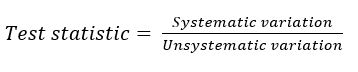
Ideally, we want a large amount of systematic variation and a small amount of unsystematic variation, so that in the end we get a large value for our test statistic. That unsystematic variation is what is also known as error variance, and is caused by nuisance variables. So we need to minimize the influence of nuisance variables on our dependent variable, as much as possible. By minimizing the variability within groups, we will have a more powerful design. So, error variance (and our ability to minimize it by controlling nuisance variables) is important for power.
For example, compare the following two, different datasets (“Low power” is one study and “High power” is another study) for our new year’s resolutions study. The scores represent the number of times each participant (n = 6 per group – yes, that is a low sample size, which is problematic for many reasons, but it works for the purposes of this particular demonstration) went to the gym in the month of January:
| Low power | High power | |||
|---|---|---|---|---|
| Wrote | Thought | Wrote | Thought | |
| 5 | 2 | 12 | 7 | |
| 18 | 5 | 13 | 7 | |
| 7 | 4 | 13 | 8 | |
| 16 | 14 | 14 | 7 | |
| 13 | 10 | 13 | 7 | |
| 19 | 7 | 13 | 6 | |
On the left, we have a dataset with low power and on the right we have a dataset with high power. In the low power scenario, you’ll notice by glancing over the numbers that there is no obvious difference in gym attendance between folks who wrote about their new year’s resolutions compared to those who simply thought about them. However, in the high power dataset, the difference between the groups jumps out at you – it is easy to see just at a glance that the people who wrote about their new year’s resolutions scored, on average, higher than those who thought about them.
Let’s take a look at some basic descriptive statistics for each of these scenarios:
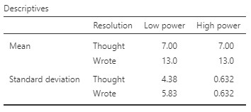
You’ll notice that the means for the Thought and Wrote group are actually the same for the low and high power datasets! However, the standard deviations are much larger in the low power dataset compared to the high power dataset. This is due to error variance: when we have a lot of error variance, it is like listening to the radio when there is a lot of static – it is hard to detect the signal from the noise. When error variance is low, the differences ‘pop out’ at you, and in those cases we have high power. Let’s run the t-test and see what that shows us:
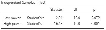
Notably, the p-value is well below .05 in the high power scenario (we would say that there is a significant difference between the groups), but not in the low power scenario. So, controlling for those nuisance variables in order to reduce error variance matters!
Of course, don’t forget that we also want to reduce the presence of confounds. Confounds are a special form of extraneous variable that systematically vary along with our independent variable – so their effects on the dependent variable are actually captured in the “systematic variation” part of our general equation for the test statistic above. They can inflate the value of the test statistic, making it look like there is an effect of the independent variable on the dependent variable when really there is not!
Error Variance: What To Do About It
Here are two general things we can do, regardless of our design, to reduce error variance:
- Use controlled conditions: in other words, keep everything constant except for the variable we are manipulating; and
- Use reliable measures.
There are also some more specific things we can do about error variance that depend on the type of design we have.
Between- or Within-Subjects Design?
One major consideration is whether to use a between-subjects or within-subjects design.
In the between-subjects design, participants would only take part in one level of the independent variable. In the within-subjects design, all participants take part in both levels.
The table below shows some other names you might hear for these two types of designs:
| Between-subjects | Within-subjects |
| Independent samples
Independent groups |
Dependent samples
Dependent groups Repeated measures |
You might hear these described as independent samples (between) or dependent samples (within). In the first case, scores in the two conditions are independent of one another, because different participants contribute to the scores in the different conditions. In the second case, the scores are dependent, or associated with each other, because the same participants contribute to the scores in the two conditions.
Now, depending on which design you use, there are different potential confounds to consider and different ways to control for extraneous variables.
Strategies for Between-Subjects Designs
There are three general tricks to dealing with extraneous variables in the between-subjects design:
- Random assignment of participants to condition:
- This does not guarantee equivalent groups but reduces the risk of confounds due to selection differences.
- Balancing participant variables: for example, in our new year’s resolution example, we might first ask how close people live to the gym, and then randomly assign them to each condition while simultaneously ensuring an even distribution of people who live close (e.g., < 1k) or far (e.g., >= 1k) from the gym in each group.
- This reduces the likelihood of participants with particular characteristics being more prevalent in one group or another when participants are randomly assigned – i.e., the extraneous variable is still present in the dataset, but will not become a confound.
- Limit the population: for example, we might limit the study to people who first report that they prefer going to the gym over other forms of exercise
- This eliminates the extraneous variable in question (but reduces external validity).
Within-Subjects Designs
If the between-subjects design is not adequately controlling extraneous variables, we can go to a within-subjects design. One approach is to use a matched-groups design. In this design, people are matched, in pairs, on one or more variable (e.g., age, distance to gym, current level of fitness, in our new year’s resolution example) and then randomly assigned from each pair to one of the two groups. It involves different participants in each group, but because those participants are matched we treat it like a within-subjects design when it comes to data analysis. This approach helps control for nuisance variables that can vary across conditions and mask the effect of the independent variable.
An ideal form of matching is to go to a full within-subjects (repeated measures) design. In this case, all participants take part in both conditions. This has the advantage of fully controlling for extraneous variables, because each participant serves as their own control. Any differences between the two conditions cannot be attributed to participant variables because they are the same participants in each condition. It is therefore an ideal form of matching.
If we are going to use a within-subjects design, we need to ensure that we use counterbalancing, otherwise, the order of conditions is a potential confound. In other words, we vary the order of exposure to the levels of the independent variable. Let’s say we have condition A and B. Half the participants would be exposed to condition A, then B, and the other half of the participants would be exposed to condition B, then A.
Caveat: of course, we cannot always use a within-subjects design. For example, a within-subjects design would not work if we wanted to test the effects of a new anxiety intervention on test anxiety, compared to a no intervention condition. The demand characteristics would likely be high, and participants would not be able to “unlearn” the effects of the anxiety intervention when they take part in the control condition. Also, within-subjects designs are more likely to result in fatigue (because the experiment will be twice as long) and have added potential confounds (e.g., practice effects) to consider.
Between or Within?
There are lots of things to consider when choosing a design. You should always weigh up the pros and cons of each design – and choosing between a between- or within-subjects design is a critical part of this process. One extra consideration is power: all other things being equal, power will be higher for the within-subjects design, because you will have the best control over participant variables in this case.
